Computational Economics: Optimization I
Florian Oswald Sciences Po, 2019
- This lecture reminds you of some optimization theory.
- The focus here is to illustrate use cases with julia.
- We barely scratch the surface of optimization, and I refer you to Nocedal and Wright for a more thorough exposition in terms of theory.
- This 2-part lecture is heavily based on Algorithms for Opimization by Kochenderfer and Wheeler.
The Optimization Process
1. Problem Specification
2. Initial Design
3. Optimization Proceedure:
    a) Evaluate Performance
    b) Good?
        i. yes: final design
        ii. no:
            * Change design
            * go back to a)
We want to automate step 3.
Optimization Algorithms
- All of the algorithms we are going to see employ some kind of iterative proceedure.
- They try to improve the value of the objective function over successive steps.
- The way the algorithm goes about generating the next step is what distinguishes algorithms from one another.
- Some algos only use the objective function
- Some use both objective and gradients
- Some add the Hessian
- and many variants more
Desirable Features of any Algorithm
- Robustness: We want good performance on a wide variety of problems in their class, and starting from all reasonable starting points.
- Efficiency: They should be fast and not use an excessive amount of memory.
- Accuracy: They should identify the solution with high precision.
A Word of Caution
- You should not normally attempt to write a numerical optimizer for yourself.
- Entire generations of Applied Mathematicians and other numerical pro's have worked on those topics before you, so you should use their work.
- Any optimizer you could come up with is probably going to perform below par, and be highly likely to contain mistakes.
- Don't reinvent the wheel.
- That said, it's very important that we understand some basics about the main algorithms, because your task is to choose from the wide array of available ones.
Optimisation Basics
- Recall our generic definition of an optimization problem:
- $x$ is our choice variable or a design point.
- $\mathcal{X}$ is the feasible set.
- $f$ is the objective function
- A vector $x^*$ is a solution or a minimizer to this problem if $x^*$ is feasible and $x^*$ minimizes $f$.
- Maximization is just minimizing $(-1)f$:
Local Solutions
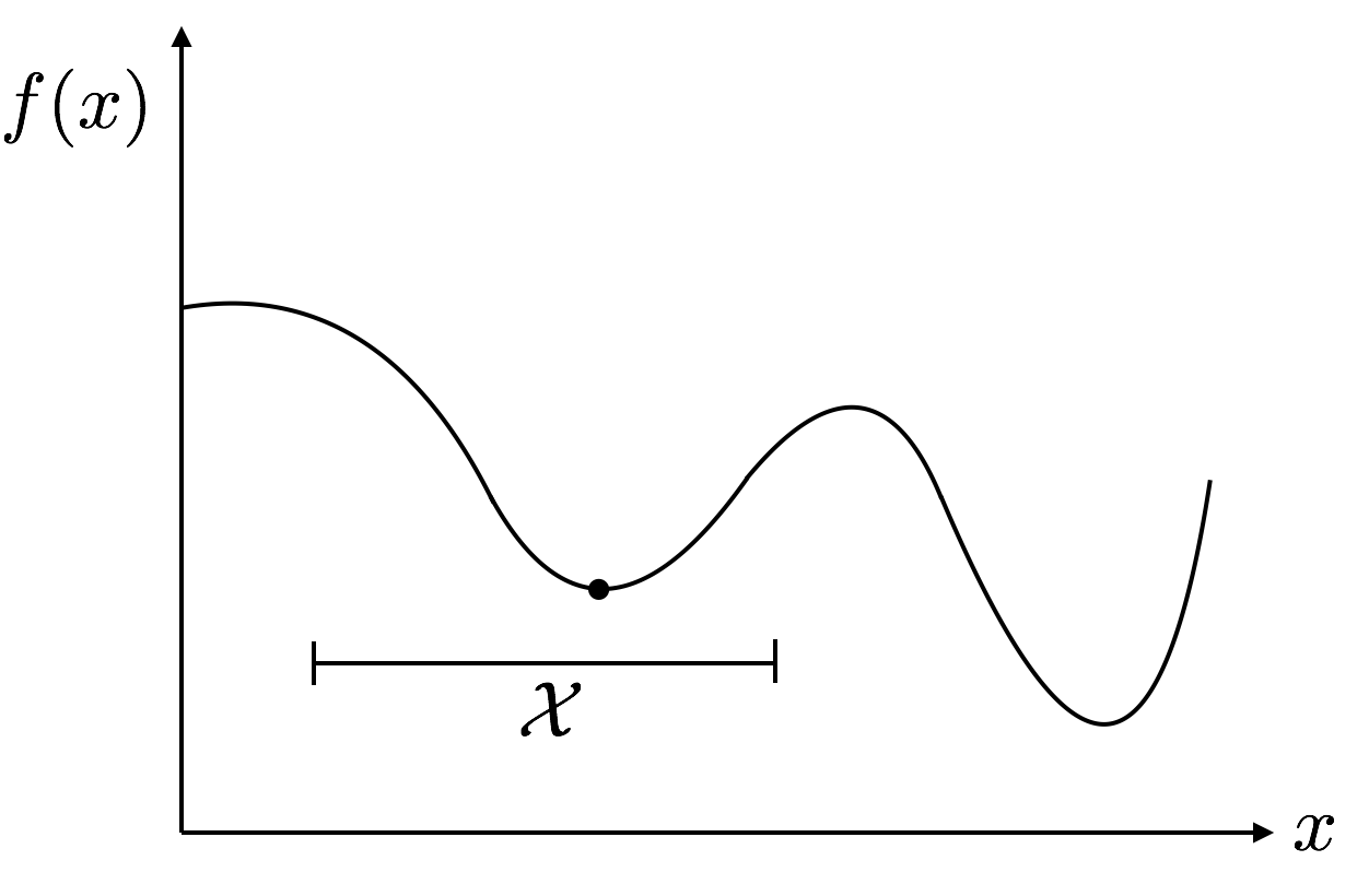
- Keep in mind that there may be other (better!) solutions outside of your interval of attention.
Constraints
- We often have constraints on problems in economics.
- Constraints define the feasible set $\mathcal{X}$.
- It's better to write weak inequalities (i.e. $\leq$) rather than strict ones ($<$).
Critical Points
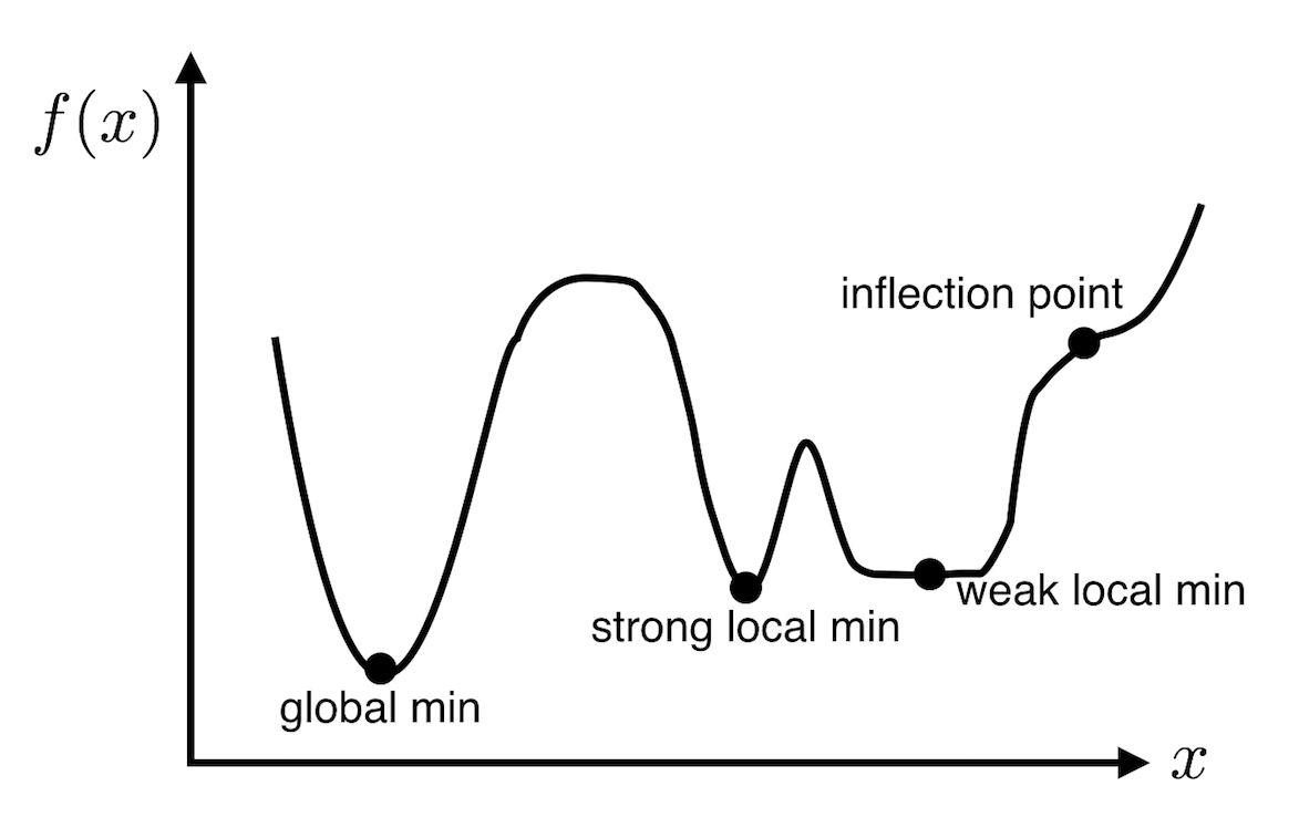
- A given univariate function can exhibit several critical points i.e. points where the derivative is zero (as we'll see).
- Ideally we would like to find a global minimum. However, that's not always straightforward to do.
- Most of the times, the best we can do is check for a local minimum
Conditions for Local Minima
We can define first and second order necessary conditions, FONC and SONC. This definition is to point out that those conditions are not sufficient for optimality (only necessary).
Univariate $f$
- FONC: $f'(x^*) =0$
- SONC $f''(x^*) \geq 0$ (and $f''(x^*) \leq 0$ for local maxima)
- (SOSC $f''(x^*) > 0$ (and $f''(x^*) < 0$ for local maxima))
Multivariate $f$
- FONC: $\nabla f(x^*) =0$
- SONC $\nabla^2f(x^*)$ is positive semidefinite (negative semidefinite for local maxima)
- (SOSC $\nabla^2f(x^*)$ is positive definite (negative definite for local maxima))
using Plots
gr()  # used to choose plotlyjs backend, but does not survive html export...
v=collect(range(-2,stop = 2, length = 30))  # values
mini = [x^2 + y^2 for x in v, y in v]
maxi = -mini   # max is just negative min
saddle = [x^2 + y^3 for x in v, y in v];
surface(v,v,maxi,title="local max",fillalpha=0.5,leg=false,fillcolor=:heat)
surface(v,v,mini,title="local min",fillalpha=0.5,leg=false,fillcolor=:heat)
surface(v,v,saddle,title="saddle",fillalpha=0.7,leg=false,fillcolor=:heat)
Example Time: Rosenbrock's Banana Function
A well-known test function for numerical optimization algorithms is the Rosenbrock banana function developed by Rosenbrock in 1960. it is defined by
$$ f(\mathbf{x}) = (1-x_1)^2 + 5(x_2-x_1^2)^2 $$# let's get a picture of this
rosenbrock(x; a=1, b=5) = (a-x[1])^2 + b*(x[2] - x[1]^2)^2
x=y=collect(range(-2,stop = 2, length = 100)) # x and y axis
f = [rosenbrock([ix,iy]) for ix in x, iy in y] # f evaluations
# plotting
wireframe(x,y,f,linecolor=:grey)
surface!(x,y,f,fillcolor=:darkrainbow,colorbar=false)
Analysing the Rosenbrock function
$$f(\mathbf{x}) = (1-x_1)^2 + 5(x_2-x_1^2)^2$$- Is the point $(1,1)$ satisfying FONC and SONC?
- Let's write down gradient and hessian to find out!
Derivatives and Gradients
- The derivative of a univariate function $f$ at point $x$, $f'(x)$ gives the rate at which $f$ changes at $x$.
- Think of a tangent line to a curve.
- There are three different ways to present $f'$: forward difference, central difference, and backward difference: $$ f'(x) \equiv \underbrace{\lim_{h\to0}\frac{f(x+h)-f(x)}{h}}_{\text{forward diff}}= \underbrace{\lim_{h\to0}\frac{f(x+h/2)-f(x-h/2)}{h}}_{\text{central diff}}=\underbrace{\lim_{h\to0}\frac{f(x)-f(x-h)}{h}}_{\text{backward diff}}$$
Symbolic Differentiation on a Computer
- If you can write down an analytic form of $f$, there are ways to symbolically differentiate it on a computer.
- This is as if you would do the derivation on paper.
- Mathematica, python, and julia all have packages for that.
- While this works well, most of the times we don't have an analytic $f$.
using SymEngine
x = symbols("x");
f = x^2 + x/2 - sin(x)/x; diff(f, x)
1/2 + 2*x + sin(x)/x^2 - cos(x)/x
Multiple Dimensions: Gradients
- Unless otherwise noted, we have $x \in \mathbb{R}^n$ as an $n$ element vector.
- The gradient of a function $f : \mathbb{R}^n \mapsto \mathbb{R}$ is denoted $\nabla f:\mathbb{R}^n \mapsto \mathbb{R}^n$ and it returns a vector
- It's hessian is a function denoted $\nabla^2 f(x)$ or $H_f :\mathbb{R}^n \mapsto \mathbb{R}^{n\times n}$ and returns an $(n,n)$ matrix given by
- The directional derivative $\nabla_s f(\mathbf{x})$ is an important concept that we will re-encounter when talking about gradient descent.
- $\nabla_s f(\mathbf{x})$ tells us the rate of change in $f$ as we move through $\mathbf{x}$ at velocity $\mathbf{s}$
- It has similiar defintion $$\nabla_s f(\mathbf{x}) \equiv \underbrace{\lim_{h\to0}\frac{f(\mathbf{x}+h\mathbf{s})-f(\mathbf{x})}{h}}_{\text{forward diff}}= \underbrace{\lim_{h\to0}\frac{f(\mathbf{x}+h/2\mathbf{s})-f(\mathbf{x}-h/2\mathbf{s})}{h}}_{\text{central diff}}=\underbrace{\lim_{h\to0}\frac{f(\mathbf{x})-f(\mathbf{x}-h\mathbf{s})}{h}}_{\text{backward diff}}$$
- We can use the gradient $\nabla f(\mathbf{x})$ to compute it: $$\nabla_\mathbf{s} f(\mathbf{x}) = \nabla f(\mathbf{x})^\top \mathbf{s}$$
For example, let's compute it for $f(\mathbf{x}) = x_1 x_2$ at $\mathbf{x} = [2, 0]$ in direction $\mathbf{s}=[-1,-1]$
$$ \begin{aligned} \nabla f(\mathbf{x}) & = \left[ ,\frac{\partial f(\mathbf{x})}{\partial x_1},\frac{\partial f(\mathbf{x})}{\partial x_2} \right] = [x_2,x_1 ] \\ \nabla_\mathbf{s} f(\mathbf{x}) & = \nabla f(\mathbf{x})^\top \mathbf{s} = \left[\begin{array}{cc}0& 2\end{array}\right] \left[\begin{array}{c}-1\\-1\end{array} \right] = -2 \end{aligned} $$
Numerical Differentiation
- In most cases we have to compute the derivative numerically. There are 2 strategies:
- Finite Differences
- Automatic Differentiation
Finite Differences
The idea here is to literally take our definition for a derivative from above, and compute it for small $h$: $$ f'(x) \approx \underbrace{\frac{f(x+h)-f(x)}{h}}_{\text{forward diff}}= \underbrace{\frac{f(x+h/2)-f(x-h/2)}{h}}_{\text{central diff}}=\underbrace{\frac{f(x)-f(x-h)}{h}}_{\text{backward diff}}$$
- The central difference has a quadratic error, as opposed to the forward difference method, hence it's often preferrable
- There is however the problem of numerical instability due to a too small $h$.
- The complex step method takes a step in an imaginary direction to bypass this: $$ f'(x) = \frac{\text{Im}(f(x+ih))}{h} + O(h^2) \text{ as }h\to \infty $$
Finite Differences: what's the right step size $h$?
- Theoretically, we would like to have $h$ as small as possible, since we want to approximate the limit at zero.
- In practice, on a computer, there is a limit to this. There is a smallest representable number, as we know.
eps().- One can show that the optimal step size is $h=\sqrt{\texttt{eps()}}$
# the Calculus.jl package implements finite differences
using Calculus

derivative(x->x^2,1.0)  # standard signature of function
println("forward = $(Calculus.finite_difference(x->x^2,1.0,:forward))")
println("central = $(Calculus.finite_difference(x->x^2,1.0,:central))")
println("complex = $(Calculus.finite_difference(x->x^2,1.0,:complex))")
println("")
println("forward = $(Calculus.finite_difference( x->sin(x^2) ,π/2,:forward))")
println("central = $(Calculus.finite_difference( x->sin(x^2) ,π/2,:central))")
println("complex = $(Calculus.finite_difference( x->sin(x^2) ,π/2,:complex))")
forward = 2.000000014901161
central = 1.9999999999829379
complex = 2.0

forward = -2.45424963163794
central = -2.4542495409833656
complex = -2.4542495411512917
# also can compute gradients for multidim functions
Calculus.gradient(x->x[1]^2 * exp(3x[2]),ones(2))
Calculus.hessian(x->x[1]^2 * exp(3x[2]),ones(2))
2×2 Array{Float64,2}:
  40.171  120.513
 120.513  180.77
# there is another problem apart from numerical issues with small h:
f1 = function(x)
    println("evaluation of f1")
    x[1]^2 * exp(3x[2])
end
Calculus.gradient(f1,ones(2))

# for an f that is expensive to compute, this method quickly becomes infeasible.
evaluation of f1
evaluation of f1
evaluation of f1
evaluation of f1
2-element Array{Float64,1}:
 40.17107384604091
 60.25661077199484
Automatic Differentiation (AD)
- Breaks down the actual
codethat defines a function and performs elementary differentiation rules, after disecting expressions via the chain rule: $$\frac{d}{dx}f(g(x)) = \frac{df}{dg}\frac{dg}{dx}$$ - This produces analytic derivatives, i.e. there is no approximation error.
- Very accurate, very fast.
- The idea is to be able to unpick expressions in your code.
- Let's look at an example
Consider the function $f(x,y) = \ln(xy + \max(x,2))$. Let's get the partial derivative wrt $x$:
$$ \begin{aligned} \frac{\partial f}{\partial x} &= \frac{1}{xy + \max(x,2)} \frac{\partial}{\partial x}(xy + \max(x,2)) \\ &= \frac{1}{xy + \max(x,2)} \left[\frac{\partial(xy)}{\partial x} + \frac{\partial\max(x,2)}{\partial x} \right]\\ &= \frac{1}{xy + \max(x,2)} \left[\left(y\frac{\partial(x)}{\partial x} + x\frac{\partial(y)}{\partial x}\right) + \left(\mathbf{1}(2>x)\frac{\partial 2}{\partial x} + \mathbf{1}(2<x)\frac{\partial x}{\partial x} \right)\right] \\ &= \frac{1}{xy + \max(x,2)} \left[y + \mathbf{1}(2<x)\right] \end{aligned} $$where the indicator function $\mathbf{1}(r)=1$ if $r$ evaluates to true, 0 otherwise.
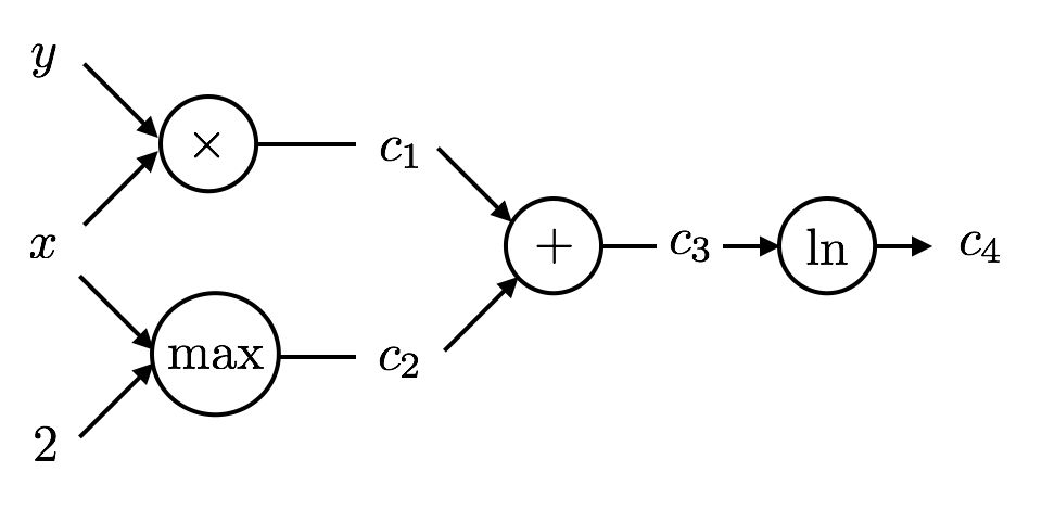
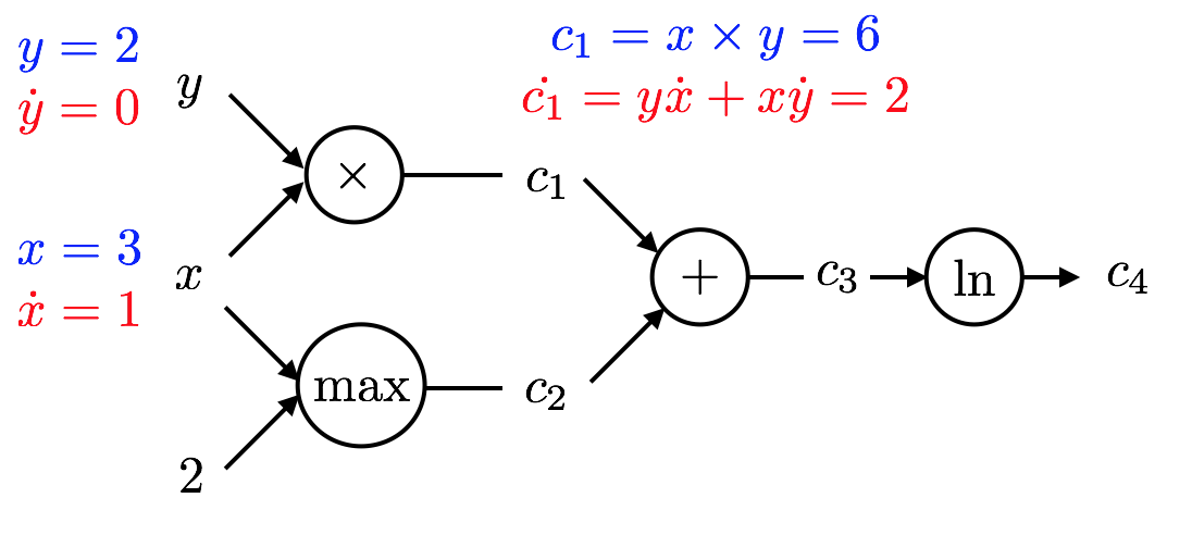
- What we just did here, i.e. unpacking the mathematical operation $\frac{\partial f}{\partial x}$ can be achieved by a computer using a computational graph.
- Automatic Differentiation traverses the computational graph of an expression either forwards (in forward accumulation mode), or backwards (in reverse accumulation mode).
This can be illustrated in a call graph as below:
- circles denote operators
- arrows are input/output
- We want to unpack the expression by successively applying the chain rule: $$ \frac{d f}{d x} = \frac{d f}{d c_4}\frac{d c_4}{d x} = \frac{d f}{d c_4}\left(\frac{d c_4}{d c_3}\frac{d c_3}{d x}\right) = \frac{d f}{d c_4}\left(\frac{d c_4}{d c_3}\left(\frac{d c_3}{d c_2}\frac{d c_2}{d x}\right)\right) = \dots $$
- Here is our operation $f(x,y)$ described as a call graph:
Accumulating forwards along the call graph
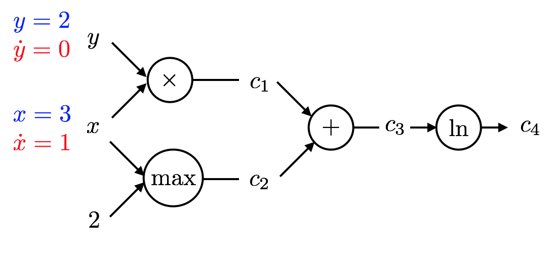
- Let's illustrate how AD in forward mode works for $x=3,y=2$ and the example at hand. Remember that $$f(x,y) = \ln(xy + \max(x,2))$$ and, hence $$f(3,2) = \ln( 6 + 3 ) = \ln 9 \text{ and }\frac{\partial f}{\partial x} = \frac{1}{6 + 3}(2 + 1) = \frac{1}{3}$$
- We start at the left side of this graph with the inputs.
- The key is for each quantity to compute both the value and it's partial derivative wrt $x$ in this case.
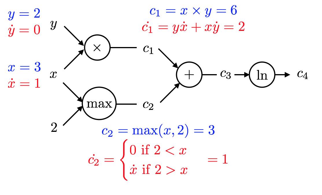
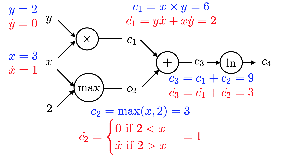
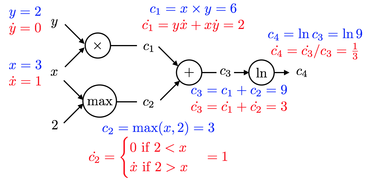
- Reverse mode works very similarly.
- So, we saw that AD yields both a function value ($c_4$) as well as a derivative ($\dot{c_4}$)
- They have the correct values.
- This procedure required a single pass forward over the computational graph.
- Notice that the exact same amount of computation needs to be performed by any program trying to evaluate merely the function value $f(3,2)$:
- multiply 2 numbers
- max of 2 numbers
- add 2 numbers
- natural logarithm of a number
QUESTION: WHY HAVE WE NOT BEEN DOING THIS FOR EVER?! ANSWER: Because it was tedious.
Implementing AD
What do you need to implement AD?
We need what is called dual numbers. This is similar to complex numbers, in that each number has 2 components: a standard value, and a derivative
- In other words, if $x$ is a dual number, $x = a + b\epsilon$ with $a,b \in \mathbb{R}$.
- For our example, we need to know how to do addition, multiplication, log and max for such a number type: $$ \begin{aligned} (a+b\epsilon) + (c+d\epsilon) &= (a+c) + (b+d\epsilon) \\ (a+b\epsilon) \times (c+d\epsilon) &= (ac) + (ad+bd\epsilon) \end{aligned} $$
- You need a programming language where analyzing expressions is not too difficult to do. you need a language that can do introspection.
Implementing Dual Numbers in Julia
This is what it takes to define a Dual number type in julia:
struct Dual
    v
    ∂
end

Base.:+(a::Dual, b::Dual) = Dual(a.v + b.v, a.∂ + b.∂)
Base.:*(a::Dual, b::Dual) = Dual(a.v * b.v, a.v*b.∂ + b.v*a.∂)
Base.log(a::Dual) = Dual(log(a.v), a.∂/a.v)
function Base.max(a::Dual, b::Dual)
    v = max(a.v, b.v)
    ∂ = a.v > b.v ? a.∂ : a.v < b.v ? b.∂ : NaN
    return Dual(v, ∂)
end
function Base.max(a::Dual, b::Int)
    v = max(a.v, b)
    ∂ = a.v > b ? a.∂ : a.v < b ? 1 : NaN
    return Dual(v, ∂)
end
# ForwardDiff.jl is a julia package for ... Forward AD!
using ForwardDiff
x = ForwardDiff.Dual(3,1);
y = ForwardDiff.Dual(2,0);
log(x*y + max(x,2))
Dual{Nothing}(2.1972245773362196,0.3333333333333333)
Analyzing Expressions
- Everything you type into julia is an
Expression:
mutable struct Expr <: Any

  Fields:

  head :: Symbol
  args :: Array{Any,1}
  typ  :: Any
println("create an explicit expression by `quoting` it with `:`")
expr = :(x + y)
println("typeof(expr)=$(typeof(expr))")

println("\ncan evaluate an expression")
x = 2;y=3
println(eval(expr))

println("\nand we can pick it apart:")
println("expr.head=$(expr.head)")
println("expr.args=$(expr.args)")
create an explicit expression by `quoting` it with `:`
typeof(expr)=Expr

can evaluate an expression
5

and we can pick it apart:
expr.head=call
expr.args=Any[:+, :x, :y]
# our example was
ex = :(log(x*y + max(x,2)))
# we can access every piece of the call graph, e.g.
println("the first elemt of args is $(ex.args[1])")

println("let's dump the entire callgraph")
dump(ex)
the first elemt of args is log
let's dump the entire callgraph
Expr
  head: Symbol call
  args: Array{Any}((2,))
    1: Symbol log
    2: Expr
      head: Symbol call
      args: Array{Any}((3,))
        1: Symbol +
        2: Expr
          head: Symbol call
          args: Array{Any}((3,))
            1: Symbol *
            2: Symbol x
            3: Symbol y
        3: Expr
          head: Symbol call
          args: Array{Any}((3,))
            1: Symbol max
            2: Symbol x
            3: Int64 2
(Unconstrained) Optimization in Julia
- Umbrella Organisation:
http://www.juliaopt.org- We will make ample use of this when we talk about constrained optimsation.
- The Julia Interface to the very well established C-Library NLopt is called
NLopt.jl. One could useNLoptwithout constraints in an unconstrained problem.
Roots.jl: Simple algorithms that find the zeros of a univariate function.- Baseline Collection of unconstrained optimization algorithms:
Optim.jl
# let's optimize rosenbrock's function without any gradient/hessian info:
using Optim
rosenbrock(x) =  (1.0 - x[1])^2 + 100.0 * (x[2] - x[1]^2)^2
result = optimize(rosenbrock, zeros(2), BFGS())
Results of Optimization Algorithm
 * Algorithm: BFGS
 * Starting Point: [0.0,0.0]
 * Minimizer: [0.9999999926033423,0.9999999852005353]
 * Minimum: 5.471433e-17
 * Iterations: 16
 * Convergence: true
   * |x - x'| ≤ 0.0e+00: false
     |x - x'| = 3.47e-07
   * |f(x) - f(x')| ≤ 0.0e+00 |f(x)|: false
     |f(x) - f(x')| = 1.20e+03 |f(x)|
   * |g(x)| ≤ 1.0e-08: true
     |g(x)| = 2.33e-09
   * Stopped by an increasing objective: false
   * Reached Maximum Number of Iterations: false
 * Objective Calls: 53
 * Gradient Calls: 53
now let's supply both hessian and gradient
- What are gradient and hessian of this function?
- Write them down on a piece of paper!
function g!(G, x)
           G[1] = -2.0 * (1.0 - x[1]) - 400.0 * (x[2] - x[1]^2) * x[1]
           G[2] = 200.0 * (x[2] - x[1]^2)
end
function h!(H, x)
           H[1, 1] = 2.0 - 400.0 * x[2] + 1200.0 * x[1]^2
           H[1, 2] = -400.0 * x[1]
           H[2, 1] = -400.0 * x[1]
           H[2, 2] = 200.0
end
optimize(rosenbrock, g!, h!, zeros(2), Newton())
Results of Optimization Algorithm
 * Algorithm: Newton's Method
 * Starting Point: [0.0,0.0]
 * Minimizer: [0.9999999999999994,0.9999999999999989]
 * Minimum: 3.081488e-31
 * Iterations: 14
 * Convergence: true
   * |x - x'| ≤ 0.0e+00: false
     |x - x'| = 3.06e-09
   * |f(x) - f(x')| ≤ 0.0e+00 |f(x)|: false
     |f(x) - f(x')| = 3.03e+13 |f(x)|
   * |g(x)| ≤ 1.0e-08: true
     |g(x)| = 1.11e-15
   * Stopped by an increasing objective: false
   * Reached Maximum Number of Iterations: false
 * Objective Calls: 44
 * Gradient Calls: 44
 * Hessian Calls: 14