Numerical Dynamic Programming
Florian Oswald, Sciences Po, 2019
Intro
- Numerical Dynamic Programming (DP) is widely used to solve dynamic models.
- You are familiar with the technique from your core macro course.
- We will illustrate some ways to solve dynamic programs.
- Models with one discrete or continuous choice variable
- Models with several choice variables
- Models with a discrete-continuous choice combination
- We will go through:
- Value Function Iteration (VFI)
- Policy function iteration (PFI)
- Projection Methods
- Endogenous Grid Method (EGM)
- Discrete Choice Endogenous Grid Method (DCEGM)
Dynamic Programming Theory
Payoffs over time are $$U=\sum_{t=1}^{\infty}\beta^{t}u\left(s_{t},c_{t}\right) $$ where $\beta<1$ is a discount factor, $s_{t}$ is the state, $c_{t}$ is the control.
The state (vector) evolves as $s_{t+1}=h(s_{t},c_{t})$.
- All past decisions are contained in $s_{t}$.
Assumptions
- Let $c_{t}\in C(s_{t}),s_{t}\in S$ and assume $u$ is bounded in $(c,s)\in C\times S$.
- Stationarity: neither payoff $u$ nor transition $h$ depend on time.
- Write the problem as $$ v(s)=\max_{s'\in\Gamma(s)}u(s,s')+\beta v(s') $$
- $\Gamma(s)$ is the constraint set (or feasible set) for $s'$ when the current state is $s$
Existence
Theorem. Assume that $u(s,s')$ is real-valued, continuous, and bounded, that $\beta\in(0,1)$, and that the constraint set $\Gamma(s)$ is nonempty, compact, and continuous. Then there exists a unique function $v(s)$ that solves the above functional equation.
Proof. [@stokeylucas] theoreom 4.6.
Solution Methods
Value Function Iteration (VFI)
- Find the fix point of the functional equation by iterating on it until the distance between consecutive iterations becomes small.
- Motivated by the Bellman Operator, and it's characterization in the Continuous Mapping Theorem.
Discrete DP VFI
- Represents and solves the functional problem in $\mathbb{R}$ on a finite set of grid points only.
- Widely used method.
- Simple (+)
- Robust (+)
- Slow (-)
- Imprecise (-)
- Precision depends on number of discretization points used.
- High-dimensional problems are difficult to tackle with this method because of the curse of dimensionality.
Deterministic growth model with Discrete VFI
- We have this theoretical model:
and we employ the followign numerical approximation: $$ V(k_i) = \max_{i'=1,2,\dots,n} u(f(k_i) - k_{i'}) + \beta V(i') $$
The iteration is then on successive iterates of $V$: The LHS gets updated in each iteration!
- And it stops at iteration $r$ if $d(V^{r},V^{r-1}) < \text{tol}$
- You choose a measure of distance, $d(\cdot,\cdot)$, and a level of tolerance.
- $V^{r}$ is usually an array. So $d$ will be some kind of norm.
- maximal absolute distance
- mean squared distance
Exercise 1: Implement discrete VFI
Checklist
- Set parameter values
- define a grid for state variable $k \in [0,2]$
- initialize value function $V$
- start iteration, repeatedly computing a new version of $V$.
- stop if $d(V^{r},V^{r-1}) < \text{tol}$.
- plot value and policy function
- report the maximum error of both wrt to analytic solution
alpha     = 0.65
beta      = 0.95
grid_max  = 2  # upper bound of capital grid
n         = 150  # number of grid points
N_iter    = 3000  # number of iterations
kgrid     = 1e-2:(grid_max-1e-2)/(n-1):grid_max  # equispaced grid
f(x) = x^alpha  # defines the production function f(k)
tol = 1e-9
Analytic Solution
- If we choose $u(x)=\ln(x)$, the problem has a closed form solution.
- We can use this to check accuracy of our solution.
ab        = alpha * beta
c1        = (log(1 - ab) + log(ab) * ab / (1 - ab)) / (1 - beta)
c2        = alpha / (1 - ab)
# optimal analytical values
v_star(k) = c1 .+ c2 .* log.(k)
k_star(k) = ab * k.^alpha
c_star(k) = (1-ab) * k.^alpha
ufun(x) = log.(x)
kgrid[4]
# Bellman Operator
# inputs
# `grid`: grid of values of state variable
# `v0`: current guess of value function

# output
# `v1`: next guess of value function
# `pol`: corresponding policy function

#takes a grid of state variables and computes the next iterate of the value function.
function bellman_operator(grid,v0)

    v1  = zeros(n)     # next guess
    pol = zeros(Int,n)     # policy function
    w   = zeros(n)   # temporary vector

    # loop over current states
    # current capital
    for (i,k) in enumerate(grid)

        # loop over all possible kprime choices
        for (iprime,kprime) in enumerate(grid)
            if f(k) - kprime < 0   #check for negative consumption
                w[iprime] = -Inf
            else
                w[iprime] = ufun(f(k) - kprime) + beta * v0[iprime]
            end
        end
        # find maximal choice
        v1[i], pol[i] = findmax(w)     # stores Value und policy (index of optimal choice)
    end
    return (v1,pol)   # return both value and policy function
end


# VFI iterator
#
## input
# `n`: number of grid points
# output
# `v_next`: tuple with value and policy functions after `n` iterations.
function VFI()
    v_init = zeros(n)     # initial guess
    for iter in 1:N_iter
        v_next = bellman_operator(kgrid,v_init)  # returns a tuple: (v1,pol)
        # check convergence
        if maximum(abs,v_init.-v_next[1]) < tol
            verrors = maximum(abs,v_next[1].-v_star(kgrid))
            perrors = maximum(abs,kgrid[v_next[2]].-k_star(kgrid))
            println("Found solution after $iter iterations")
            println("maximal value function error = $verrors")
            println("maximal policy function error = $perrors")
            return v_next
        elseif iter==N_iter
            warn("No solution found after $iter iterations")
            return v_next
        end
        v_init = v_next[1]  # update guess
    end
end

# plot
using Plots
function plotVFI()
    v = VFI()
    p = Any[]

    # value and policy functions
    push!(p,plot(kgrid,v[1],
            lab="V",
            ylim=(-50,-30),legend=:bottomright),
            plot(kgrid,kgrid[v[2]],
            lab="policy",legend=:bottomright))

    # errors of both
    push!(p,plot(kgrid,v[1].-v_star(kgrid),
        lab="V error",legend=:bottomright),
        plot(kgrid,kgrid[v[2]].-k_star(kgrid),
        lab="policy error",legend=:bottomright))

    plot(p...,layout=grid(2,2) )

end

plotVFI()
Exercise 2: Discretizing only the state space (not control space)
- Same exercise, but now use a continuous solver for choice of $k'$.
- in other words, employ the following numerical approximation: $$ V(k_i) = \max_{k'\in[0,\bar{k}]} \ln(f(k_i) - k') + \beta V(k') $$
- To do this, you need to be able to evaluate $V(k')$ where $k'$ is potentially off the
kgrid. - use
Interpolations.jlto linearly interpolate V.- the relevant object is setup with function
interpolate((grid,),v,Gridded(Linear()))
- the relevant object is setup with function
- use
Optim::optimize()to perform the maximization.- you have to define an ojbective function for each $k_i$
- do something like
optimize(objective, lb,ub)
kgrid
using Interpolations
using Optim
function bellman_operator2(grid,v0)

    v1  = zeros(n)     # next guess
    pol = zeros(n)     # consumption policy function

    Interp = interpolate((collect(grid),), v0, Gridded(Linear()) )
    Interp = extrapolate(Interp,Interpolations.Flat())

    # loop over current states
    # of current capital
    for (i,k) in enumerate(grid)

        objective(c) = - (log.(c) + beta * Interp(f(k) - c))
        # find max of ojbective between [0,k^alpha]
        res = optimize(objective, 1e-6, f(k))  # Optim.jl
        pol[i] = f(k) - res.minimizer   # k'
        v1[i] = -res.minimum
    end
    return (v1,pol)   # return both value and policy function
end

function VFI2()
    v_init = zeros(n)     # initial guess
    for iter in 1:N_iter
        v_next = bellman_operator2(kgrid,v_init)  # returns a tuple: (v1,pol)
        # check convergence
        if maximum(abs,v_init.-v_next[1]) < tol
            verrors = maximum(abs,v_next[1].-v_star(kgrid))
            perrors = maximum(abs,v_next[2].-k_star(kgrid))
            println("continuous VFI:")
            println("Found solution after $iter iterations")
            println("maximal value function error = $verrors")
            println("maximal policy function error = $perrors")
            return v_next
        elseif iter==N_iter
            warn("No solution found after $iter iterations")
            return v_next
        end
        v_init = v_next[1]  # update guess
    end
    return nothing
end

function plotVFI2()
    v = VFI2()
    p = Any[]

    # value and policy functions
    push!(p,plot(kgrid,v[1],
            lab="V",
            ylim=(-50,-30),legend=:bottomright),
            plot(kgrid,v[2],
            lab="policy",legend=:bottomright))

    # errors of both
    push!(p,plot(kgrid,v[1].-v_star(kgrid),
        lab="V error",legend=:bottomright),
        plot(kgrid,v[2].-k_star(kgrid),
        lab="policy error",legend=:bottomright))

    plot(p...,layout=grid(2,2) )

end

plotVFI2()
Policy Function Iteration
- This is similar to VFI but we now guess successive policy functions
- The idea is to choose a new policy $p^*$ in each iteration so as to satisfy an optimality condition. In our example, that would be the Euler Equation.
- We know that the solution to the above problem is a function $c^*(k)$ such that
- We don't directly solve the maximiation problem outlined above, but it's first order condition:
- In practice, we have to find the zeros of
# Your turn!


using Roots
function policy_iter(grid,c0,u_prime,f_prime)

    c1  = zeros(length(grid))     # next guess
    pol_fun = extrapolate(interpolate((collect(grid),), c0, Gridded(Linear()) ) , Interpolations.Flat())


    # loop over current states
    # of current capital
    for (i,k) in enumerate(grid)
        objective(c) = u_prime(c) - beta * u_prime(pol_fun(f(k)-c)) * f_prime(f(k)-c)
        c1[i] = fzero(objective, 1e-10, f(k)-1e-10)
    end
    return c1
end

uprime(x) = 1.0 ./ x
fprime(x) = alpha * x.^(alpha-1)

function PFI()
    c_init = kgrid
    for iter in 1:N_iter
        c_next = policy_iter(kgrid,c_init,uprime,fprime)
        # check convergence
        if maximum(abs,c_init.-c_next) < tol
            perrors =  maximum(abs,c_next.-c_star(kgrid))
            println("PFI:")
            println("Found solution after $iter iterations")
            println("max policy function error = $perrors")
            return c_next
        elseif iter==N_iter
            warn("No solution found after $iter iterations")
            return c_next
        end
        c_init = c_next  # update guess
    end
end
function plotPFI()
    v = PFI()
    plot(kgrid,[v v.-c_star(kgrid)],
            lab=["policy" "error"],
            legend=:bottomright,
            layout = 2)
end
plotPFI()
Projection Methods
- Many applications require us to solve for an unknown function
- ODEs, PDEs
- Pricing functions in asset pricing models
- Consumption/Investment policy functions
- Projection methods find approximations to those functions that set an error function close to zero.
Example: Growth, again
- We stick to our working example from above.
- We encountered the Euler Equation $g$ for optimality.
- At the true consumption function $c^*$, $g(k) = 0$.
- We define the following function operator:
- The Equilibrium solves the operator equation $$ 0 = \mathcal{N}(c^*) $$
Projection Method example
create an approximation to $c^*$: find $$ \bar{c} \equiv \sum_{i=0}^n a_i k^i $$
which nearly solves
$$\mathcal{N}(c^*)=0 $$
- Compute Euler equation error function: $$ g(k;a) = u'(\bar{c}(k)) - \beta u'[\bar{c}(f(k)-\bar{c}(k))] f'(f(k)-\bar{c}(k))$$
- Choose $a$ to make $g(k;a)$ small in some sense
What's small in some sense?
- Least-squares: minimize sum of squared errors $$ \min_a \int g(k;a)^2 dk $$
- Galerkin: zero out weighted averages of Euler errors
- Collocation: zero out Euler equation errors at grid $k\in\{k_1,\dots,k_n\}$: $$ P_i(a) \equiv g(k_i;a) = 0, i=1,\dots,n $$
General Projection Method
- Express solution in terms of unknown function $$ \mathcal{N}(h)=0 $$ where $h(x)$ is the equilibrium function at state $x$
- Choose a space for appximation
- Find $\bar{h}$ which nearly solves $$ \mathcal{N}(\bar{h})=0$$
Projection method exercise
- suppose we want to find effective supply of an oligopolistic firm in cournot competition.
- We want to know $q = S(p)$, how much is supplied at each price $p$.
- This function is characterized as
- Take $D(p) = p^{-\eta}$ and $MC(q) = \alpha \sqrt{q} + q^2$.
- Our task is to solve for $S(p)$ in
- No closed form solution. But collocation works!
TASK
- solve for $S(p)$ by collocation
- Plot residual function
- Plot resulting $mS(p)$ together with market demand and $m=1,10,20$ for market size.
using CompEcon
using Plots
using NLsolve
function proj(n=25)

    alpha = 1.0
    eta   = 1.5
    a     = 0.1
    b     = 3.0
    basis = fundefn(:cheb,n,a,b)
    p     = funnode(basis)[1]   # collocation points

    c0 = ones(n)*0.3
    function resid!(c::Vector,result::Vector,p,basis,alpha,eta)
        # your turn!
        q = funeval(c,basis,p)[1]
        q2 = similar(q)
        for i in eachindex(q2)
            if q[i] < 0
                q2[i] = -20.0
            else
                q2[i] = sqrt(q[i])
            end
        end
        result[:] = p.+ q .*((-1/eta)*p.^(eta+1)) .- alpha*q2 .- q.^2
    end
    f_closure(r::Vector,x::Vector) = resid!(x,r,p,basis,alpha,eta)
    res = nlsolve(f_closure,c0)
    println(res)

    # plot residual function
     x = collect(range(a, stop = b, length = 501))
    y = similar(x)
    resid!(res.zero,y,x,basis,alpha,eta);
    y = funeval(res.zero,basis,x)[1]
    pl = Any[]
    push!(pl,plot(x,y,title="residual function"))

    # plot supply functions at levels 1,10,20

    # plot demand function
    y = funeval(res.zero,basis,x)[1]
    p2 = plot(y,x,label="supply 1")
    plot!(10*y,x,label="supply 10")
    plot!(20*y,x,label="supply 20")
    d = x.^(-eta)
    plot!(d,x,label="Demand")

    push!(pl,p2)

    plot(pl...,layout=2)

end
proj()
Endogenous Grid Method (EGM)
- Fast, elegant and precise method to solve consumption/savings problems
- One continuous state variable
- One continuous control variable $$V(M_t) = \max_{0<c<M_t} u(c) + \beta E V_{t+1}(R (M_t - c) + y_{t+1})$$
- Here, $M_t$ is cash in hand, all available resources at the start of period $t$
- For example, assets plus income.
- $A_t = M_t - c_t$ is end of period assets
- $y_{t+1}$ is stochastic next period income.
- $R$ is the gross return on savings, i.e. $R=1+r$.
- utility function can be of many forms, we only require twice differentiable and concave.
EGM after [@carroll2006method]
- [@carroll2006method] introduced this method.
- The idea is as follows:
- Instead of using non-linear root finding for optimal $c$ (see above)
- fix a grid of possible end-of-period asset levels $A_t$
- use structure of model to find implied beginning of period cash in hand.
- We use euler equation and envelope condition to connect $M_{t+1}$ with $c_t$
Recall Traditional Methods: VFI and Euler Equation
- Just to be clear, let us repeat what we did in the beginning of this lecture, using the $M_t$ notation. $$ \begin{aligned} V(M_t) &= \max_{0<c<M_t} u(c) + \beta E V_{t+1}(R (M_t - c) + y_{t+1}) \\ M_{t+1} &= R (M_t - c) + y_{t+1} \end{aligned} $$
VFI
- Define a grid over $M_t$.
- In the final period, compute $$V_T(M_T) = \max_{0<c<M_t} u(c)$$
- In all preceding periods $t$, do $$V_t(M_t) = \max_{0<c_t<M_t} u(c_t) + \beta E V_{t+1}(R (M_t - c_t) + y_{t+1})$$
- where optimal consumption is $$c_t^*(M_t) = \arg \max_{0<c_t<M_t} u(c_t) + \beta E V_{t+1}(R (M_t - c_t) + y_{t+1})$$
Euler Equation
- The first order condition of the Bellman Equation is $$ \begin{aligned} \frac{\partial V_t}{\partial c_t} & = 0 \\ u'(c_t) & = \beta E \left[\frac{\partial V_{t+1} (M_{t+1}) }{\partial M_{t+1}} \right] \quad (FOC) \end{aligned} $$
- By the Envelope Theorem, we have that $$ \begin{aligned} \frac{\partial V_t}{\partial M_t} & = \beta E \left[\frac{\partial V_{t+1} (M_{t+1}) }{\partial M_{t+1}} \right] \\ \text{by FOC} & \\ \frac{\partial V_t}{\partial M_t} & = u'(c_t) \\ \text{true in every period:} & \\ \frac{\partial V_{t+1}}{\partial M_{t+1}} & = u'(c_{t+1}) \end{aligned} $$
- Summing up, we get the Euler Equation: $$ u'(c_t) = \beta E \left[u'(c_{t+1}) R \right] $$
Euler Equation Algorithm
- Fix grid over $M_t$
- In the final period, compute $$c_T^*(M_T) = \arg\max_{0<cT<M_t} u(c_T)$$
- With optimal $c_{t+1}^*(M_{t+1})$ in hand, backward recurse to find $c_t$ from $$u'(c_t) = \beta E \left[u'(c_{t+1}^*(R (M_t - c_t) + y_{t+1}) ) R \right]$$
- Notice that if $M_t$ is small, the euler equation does not hold.
- In fact, the euler equation would prescribe to borrow, i.e. set $M_t <0$. This is ruled out.
- So, one needs to tweak this algorithm to check for this possibility
- Homework.
The EGM Algorithm
Starts in period $T$ with $c_T^* = M_T$. For all preceding periods:
- Fix a grid of end-of-period assets $A_t$
- Compute all possible next period cash-in-hand holdings $M_{t+1}$
$$ M_{t+1} = R * A_t + y_{t+1} $$
- for example, if there are $n$ values in $A_t$ and $m$ values for $y_{t+1}$, we have $dim(M_{t+1}) = (n,m)$
- Given that we know optimal policy in $t+1$, use it to get consumption at each $M_{t+1}$ $$ c_{t+1}^* (M_{t+1}) $$
- Invert the Euler Equation to get current consumption compliant with an expected level of cash-on-hand, given $A_t$ $$ c_{t} = (u')^{-1} \left( \beta E \left[u'(c_{t+1}^*(M_{t+1}) ) R |A_t \right] \right) $$
- Current period endogenous cash on hand just obeys the accounting relation $$ M_t = c_t + A_t $$
# minimal EGM implementation, go here: https://github.com/floswald/DCEGM.jl/blob/master/src/dc_algo.jl#L4
# try out:
# ] dev https://github.com/floswald/DCEGM.jl
using DCEGM
DCEGM.minimal_EGM(dplot = true);
Discrete Choice EGM
- This is a method developed by Fedor Iskhakov, Thomas Jorgensen, John Rust and Bertel Schjerning.
- Reference: [@iskhakovRust2014]
- Suppose we have several discrete choices (like "work/retire"), combined with a continuous choice in each case (like "how much to consume given work/retire").
- Let $d=0$ mean to retire.
- Write the problem of a worker as
- The problem of a retiree is
- Our task is to compute the optimal consumption functions $c_t^*(M_t|d_t=0)$, $c_t^*(M_t|d_t=1)$
Problems with Discrete-Continuous Choice
- Even if all conditional value functions $v$ are concave, the envelope over them, $V$, is in general not.
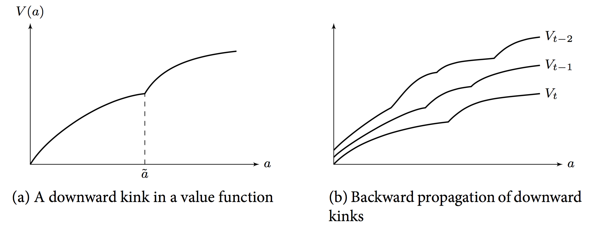
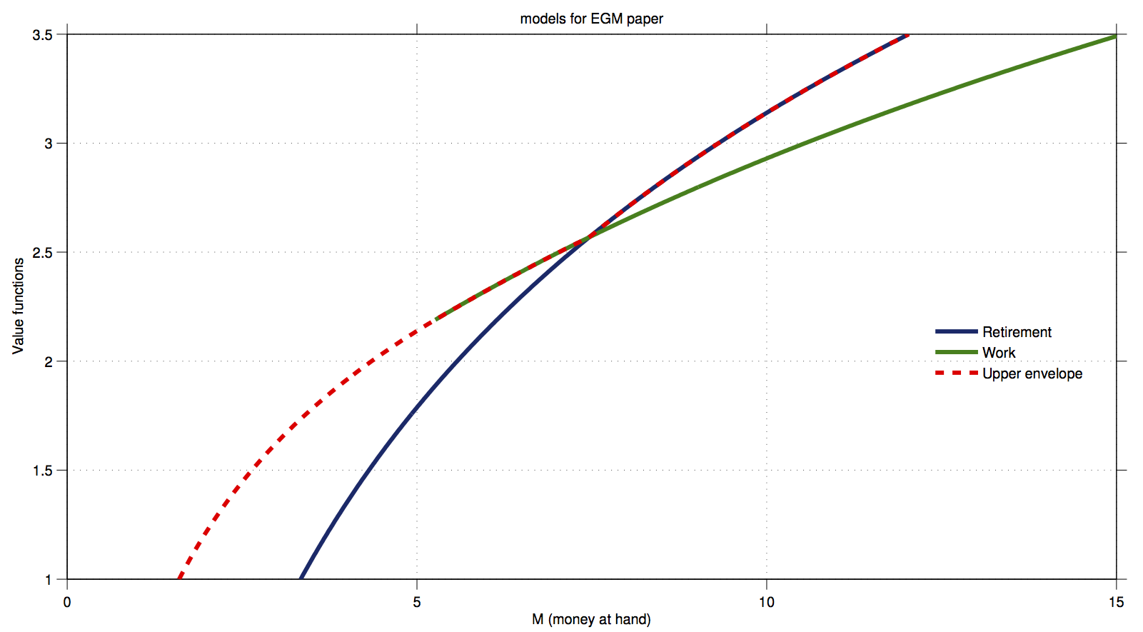
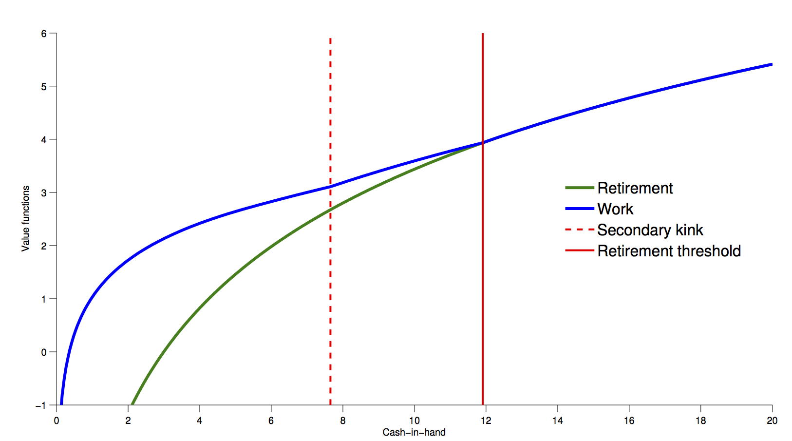
- [@clausenenvelope] show that there will be a kink point $\bar{M}$ such that
$$ v_t(\bar{M}|d_t=0) = v_t(\bar{M}|d_t=1) $$
- We call any such point a primary kink (because it refers to a discrete choice in the current period)
- $V$ is not differentiable at $\bar{M}$.
- However, it can be shown that both left and right derivatives exist, with $$ V^-(\bar{M}) < V^+(\bar{M}) $$
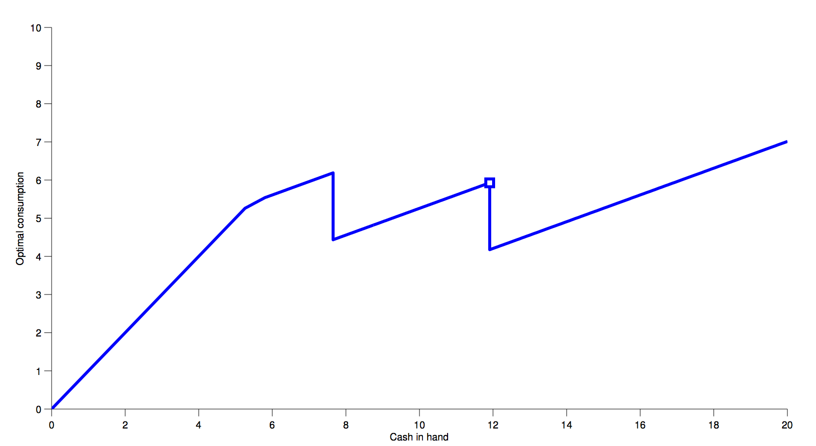
- Given that the value of the derivative changes discretely at $\bar{M_t}$, the value function in $t-1$ will exhibit a discontinuity as well:
- $v_{t-1}$ depends on $V_t$.
- Tracing out the optimal choice of $c_{t-1}$ implies next period cash on hand $M_t$, and as that hits $\bar{M_t}$, the derivative jumps.
- The derivative of the value function determines optimal behaviour via the Euler Equation.
- We call a discontinuity in $v_{t-1}$ arising from a kink in $V_t$ a secondary kink.
- The kinks propagate backwards.
- [@iskhakovRust2014] provide an analytic example where one can compute the actual number of kinks in period 1 of T.
- Figure 1 in [@clausenenvelope]:
![[@iskhakovRust2014] figure 1](../assets/figs/fedor-1.png)
Kinks
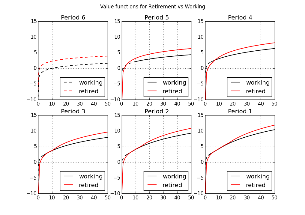
- Refer back to the work/retirement model from before.
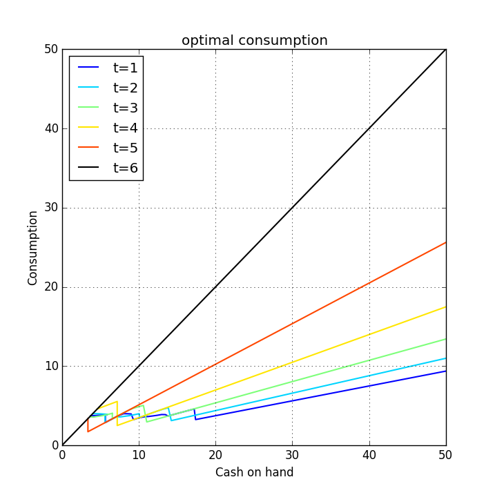
- 6 period implementation of the DC-EGM method:
Optimal consumption in 6 period model:
The Problem with Kinks
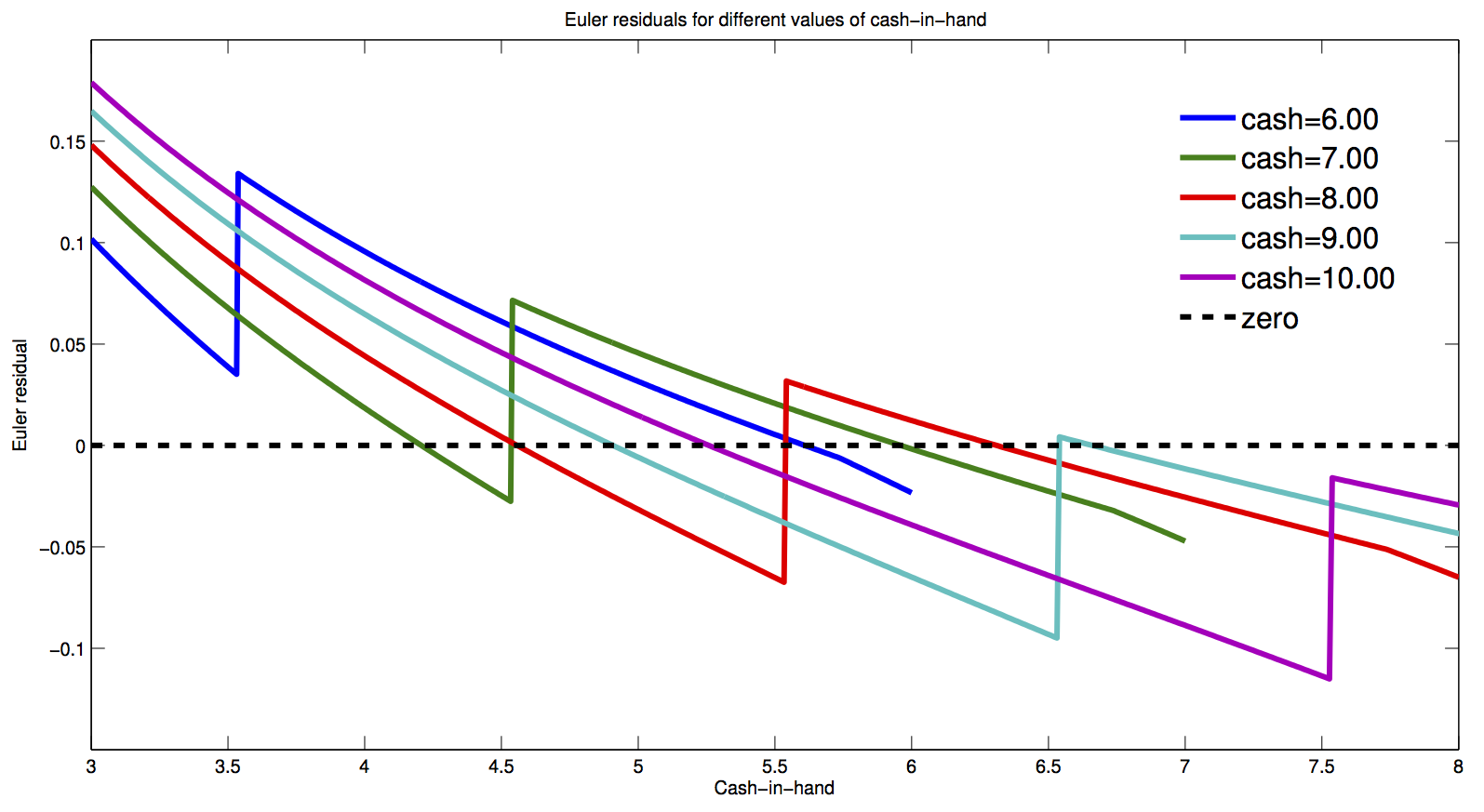
- Relying on fast methods that rely on first order conditions (like euler equation) will fail.
- There are multiple zeros in the Euler Equation, and a standard Euler Equation approach is not guaranteed to find the right one.
- picture from Fedor Iskhakov's master class at cemmap 2015:
DC-EGM Algorithm
- Do the EGM step for each discrete choice $d$
- Compute $d$-specific consumption and value functions
- compare $d$-specific value functions to find optimal switch points
- Build envelope over $d$-specific consumption functions with knowledge of which optimal $d$ applies where.
But EGM relies on the Euler Equation?!
- Yes.
- An important result in [@clausenenvelope] is that the Euler Equation is still the necessary condition for optimal consumption
- Intuition: marginal utility differs greatly at $\epsilon+\bar{M}$.
- No economic agent would ever locate at $\bar{M}$.
- This is different from saying that a proceedure that tries to find the zeros of the Euler Equation would still work.
- this will pick the wrong solution some times.
- EGM finds all solutions.
- There is a proceedure to discard the "wrong ones". Proof in [@iskhakovRust2014]
Adding Shocks
- This problem is hard to solve with standard methods.
- It is hard, because the only reliable method is VFI, and this is not feasible in large problems.
- Adding shocks to non-smooth problems is a widely used remedy.
- think of "convexifying" in game theoretic models
- (Add a lottery)
- Also used a lot in macro
- Adding shocks does indeed help in the current model.
- We add idiosyncratic taste shocks: Type 1 EV.
- Income uncertainty:
- In general, the more shocks, the more smoothing.
- The problem becomes
where the value for retirees stays the same.
Full DC-EGM
- Needs to discard false solutions.
- Criterion:
- grid in $A_t$ is increasing
- Assuming concave utility function, the function $$ A(M|d) = M - c(M|d) $$ is monotone non-decreasing
- This means that, if you go through $A_i$, and find that $$ M_t(A^j) < M_t(A^{j-1}) $$ you know you entered a non-concave region
- The Algorithm goes through the upper envelope and prunes the inferior points $M$ from the endogenous grids.
- Precise details of Algorithm in paper.
- Julia implementation on floswald/ConsProb.jl
![[@iskhakovRust2014] figure 2](../assets/figs/fedor-7.png)
![[@iskhakovRust2014] figure 4](../assets/figs/fedor-6.png)
![[@iskhakovRust2014] figure 4](../assets/figs/fedor-8.png)